Parallel Computing in R
POS6933: Computational Social Science
Truscott (Spring 2026)
Parallel Computing
Parallel Computing concerns the practice of dividing a large computational task into smaller parts that can be executed simultaneously – that is, in parallel – rather than one after another. The goal is to increase processing speeds, handle larger problems (tasks and data), and deploy resources more efficiently.
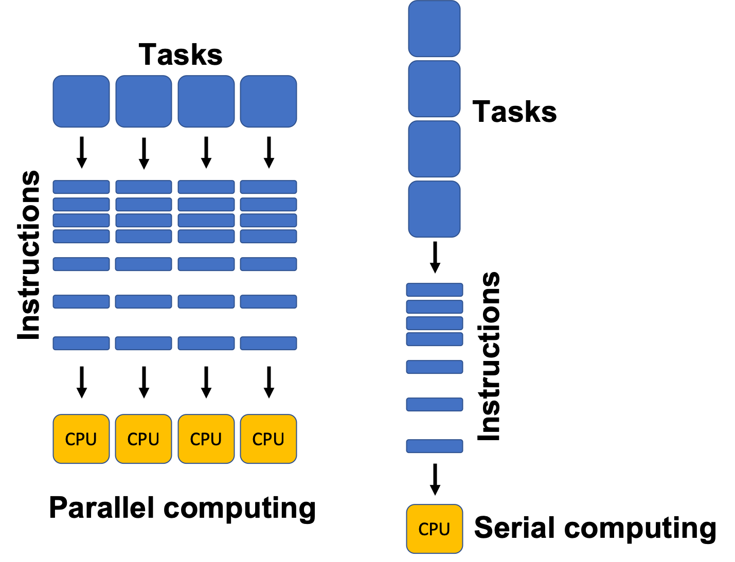
In traditional (or serial) computing, a program runs on a single processor core and executes one instruction at a time. As problems get larger or more complex (e.g., simulating electoral outcomes, training machine learning models, or otherwise processing massive datasets) this approach becomes too slow. Parallel computing solves this by spreading the work across multiple cores, processors, or even machines, allowing many operations to occur at once.
Payroll at the University of Florida (Example)
Imagine you are responsible for discharging payroll to all employees (faculty, staff, etc.) at the University of Florida. This is approximately 33,000 people – all of whom we can assume are registered for direct deposit and would very much appreciate being paid correctly and in a timely manner. For the sake of the example, let’s further assume everything with respect to payroll can be automated. However, you are responsible with designing a programming routine to actually discharge payroll – each of which requires 0.25 seconds. Using a single system, we can easily compute the completion time as:
.
Clearly not very efficient – but it’s the result of practical limitations. Traditional computers are designed to execute instructions one after another in a sequence, which can make completing large volumes of tasks a burdensome and time-consuming endeavor.
But what if we have two computers? The time to complete an independent task remains fixed (0.25 seconds/each) due to the serial constraints of the computing process, but what if we divided and allocated the tasks equally to each computer? Suddenly, the completion time has been cut in half:
.
Adding additional computers – say, 3 (About 45 Minutes), 4 (About 34 Minutes), or 5 (About 27 minutes) computers – continues to reduce the computation time. What was once a 2.3 hour task is suddenly about 30 minutes without changing the serial structure of the computing process – we just added more computers to handle the workload!
This concept is at the heart of parallel computing (generally) and
high performance computing environments like HiPerGator.
Barring quantum computing (which, please… don’t ask me about), computers
can only operationalize tasks serially, but dividing the tasks across
multiple computing units simultaneously can drastically improve
computational efficiency. Even cooler, virtually every modern laptop on
the consumer market can facilitate a parallel environment – you just
need to tell your computer (or R) to do it!
Below, I provide some key terms to understand re: parallel computing,
as well as how to set-up and deploy a parallel environment in
R
Key Terms
CPU (Central Processing Unit): The CPU is the brain of a computer. It performs calculations and executes instructions. Most modern CPUs have multiple cores, and each core can handle its own stream of instructions. This means a CPU can run several tasks in parallel. For example, a quad-core processor can process four tasks at once.
Processor vs. Core: A processor is the entire chip that fits into your computer’s motherboard (i.e., the entire CPU). A core is a general term for either a single processor on your own computer (technically you only have one processor, but a modern processor like the i7 can have multiple cores - hence the term) or a single machine in a cluster network.
Thread: A thread is the smallest sequence of instructions that a CPU can execute independently. Modern operating systems can schedule multiple threads per core, allowing one core to handle multiple tasks “concurrently” by quickly switching between them. This is sometimes called multithreading (e.g., in the UF payroll example, one thread could calculate salaries, another could generate direct deposit files, and another could send notifications – all at the same time on a multithreaded system.)
RAM (Random Access Memory): RAM is the computer’s short-term memory. It stores data that’s actively being used so the CPU can access it quickly. In parallel computing, enough RAM is crucial because multiple processors may need to access or share large amounts of data at the same time – alternatively, allocating memory independently to an individual core (or cores) helps ensure that RAM is not accidentally overburdened trying to hold onto (unnecessary) data for sevral tasks simultaneously.
Nodes: A node is a single computer in a cluster – a group of computers linked together to work on a common task. Each node has its own CPU(s), memory (RAM), and sometimes storage.
Cluster: A cluster is a collection of nodes that work together like one powerful machine. Each node handles a portion of the computation, and the results are combined at the end.
HiPerGatoris a giant computing cluster from which we can isolate “smaller” allocations of nodes and memory for complex computing tasks.
Setting Up a Parallel Environment in R
An easy way to understand what’s happening under the hood when you’re
using parallel processing in R is that for each core
you initialize (register), you’re telling it to create background
sessions to independently handle a portion of the larger
workload.
There are a handful of different means to facilitate a parallel
environment in R, and I have been fairly inconsistent in
preferring one suite of packages to initiate the start-up over another.
However, for the sake of this course, I will show you how to do it
primarily using parallel::().
suppressPackageStartupMessages({
  library(parallel);
  library(doParallel)
}) # Load Parallel (Quietly)
Recall that the CPU included in most modern computers contain several
cores, all of which allow for independent computation. Using
detectCores(), we can recover the number you have available
to you. However, a good rule of thumb – depending on how much computing
power you still need when these processes are running – is to avoid
maxing-out your core allocation for parallel tasks. For instance, if you
still wanted to be able to run R using a different project
(or maybe even just scroll on your computer…), prescribing more of your
computing resources to the parallel job reduces the resources that can
be used for other things.
Leaving at least one core available for other tasks is always
a good idea – as you will see below, I generally (at minimum) indicate
the number of cores to use as (numcores - 1).
numcores <- parallel::detectCores()
message('You Have ', numcores, ' Cores Available for Use!')
## You Have 14 Cores Available for Use!Next, we will use makeCluster() to initialize the larger
volume of available cores into a single socket cluster. Note:
There are several additional arguments to declare in
makeCluster(), virtually all of which can be ignored.
cl <- makeCluster(numcores - 1) # Create a Socket Cluster
doParallel::registerDoParallel(cl) # Register the Parallel Environment (cl)
stopCluster(cl) # Relieves Cluster
Congrats – You’ve created a parallel environment with several cores! Now, we need to actually run something. Let’s create a function with something that seems tedious but may take a moment – like 10 million draws from a standard normal distribution and we’ll subsequently calculate the mean of those squared values.
We will use lapply() to serially apply the function
serially across 10 repetitions, then do the same using
parLapply() (the parallel version) and compare the
completion times.
tedious_function <- function(x) {
  y <- rnorm(10000000) # Simulate 10 Million Draws
  mean(y^2) # Recover Mean of Squared Values
}

serial <- system.time({
  serial_run <- lapply(1:10, tedious_function)
}) # Serial Run


cl <- makeCluster(numcores - 1) # Create a Socket Cluster
doParallel::registerDoParallel(cl) # Register the Parallel Environment (cl)

parallel <- system.time({
  parallel_run <- parLapply(cl, 1:10, tedious_function)
}) # Parallel Run

stopCluster(cl) # Shut Down Parallel
## Serial Completion Time: 5.32 Seconds## Parallel Completion Time: 0.76 SecondsThe routine executed using a parallel approach is clearly faster, though evidently not by much here. However, it’s important to recognize that the most obvious benefits of parallel computing emerge when you need to engage with tasks of considerable scale – e.g., the payroll example above.
A Few Important Things to Remember
Whenever you are done using a local parallel environment, be sure to use
stopCluster()to fully and cleanly shut down the backgroundRworker processes you’ve created. If you leave a cluster running, those processes continue to consume memory and system resources, which can slow down your computer or cause errors in later parallel tasks.It’s important to view each node you’ve created with
registerDoParallelas their ownRsessions, so each one is going to need the necessary packages or libraries, as well as any objects (e.g., data, functions, etc.) stored in the global environment.
You can achieve that using a combination of clusterEvalQ
for exporting libraries and clusterExport()for objects and
functions in the global environment. Below are some examples from a
project I have been working on to simulate turnover in the American
lower federal courts – every core I create needs to have its own copy of
those items.
clusterExport(cl, c("predict_survival", 'new_judge', 'election_simulation', 'senate_moratorium', 'senate_rejection', 'single_simulation_analysis', 'electoral_outcomes_02_24', 'departure_simulation_comparison', 'd1', 'c1', 'fjc_combined_survival', 'allocated_seats', 'nominate', 'senate_rejection_data'))  # Allocate Global Environment Objects & Functions to Nodes

clusterEvalQ(cl, {
  library(dplyr)
  library(survival)
  library(stringr)
}) # Allocate Necessary Packages